Postprocessing using PyVista and Matplotlib

This example demonstrates the postprocessing capabilities of PyFluent (using PyVista and Matplotlib) using a 3D model of an exhaust manifold with high temperature flows passing through. The flow through the manifold is turbulent and involves conjugate heat transfer.

This example demonstrates postprocessing using pyvista

• Create surfaces for the display of 3D data.

• Display filled contours of temperature on several surfaces.

• Display velocity vectors.

• Plot quantitative results using Matplotlib

# sphinx_gallery_thumbnail_number = -5

import ansys.fluent.core as pyfluent
from ansys.fluent.core import examples

from ansys.fluent.visualization import set_config
from ansys.fluent.visualization.matplotlib import Plots
from ansys.fluent.visualization.pyvista import Graphics

set_config(blocking=True, set_view_on_display="isometric")

First, download the case and data file and start Fluent as a service with Solver mode, double precision, number of processors: 2

import_case = examples.download_file(
    filename="exhaust_system.cas.h5", directory="pyfluent/exhaust_system"
)

import_data = examples.download_file(
    filename="exhaust_system.dat.h5", directory="pyfluent/exhaust_system"
)

session = pyfluent.launch_fluent(
    precision="double", processor_count=2, start_transcript=False
)

session.solver.tui.file.read_case(case_file_name=import_case)
session.solver.tui.file.read_data(case_file_name=import_data)

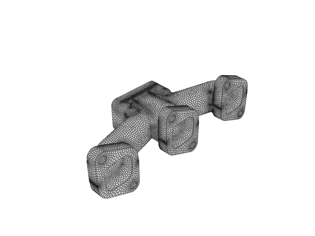
Get the graphics object for mesh display

graphics = Graphics(session=session)

Create a graphics object for mesh display

mesh1 = graphics.Meshes["mesh-1"]

Show edges

mesh1.show_edges = True

Get the surfaces list

mesh1.surfaces_list = [
    "in1",
    "in2",
    "in3",
    "out1",
    "solid_up:1",
    "solid_up:1:830",
    "solid_up:1:830-shadow",
]
mesh1.display("window-1")

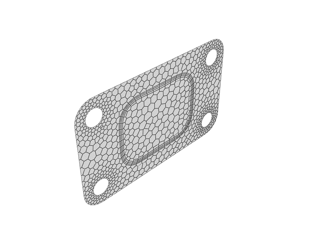
Disable edges and display again

mesh1.show_edges = False
mesh1.display("window-2")

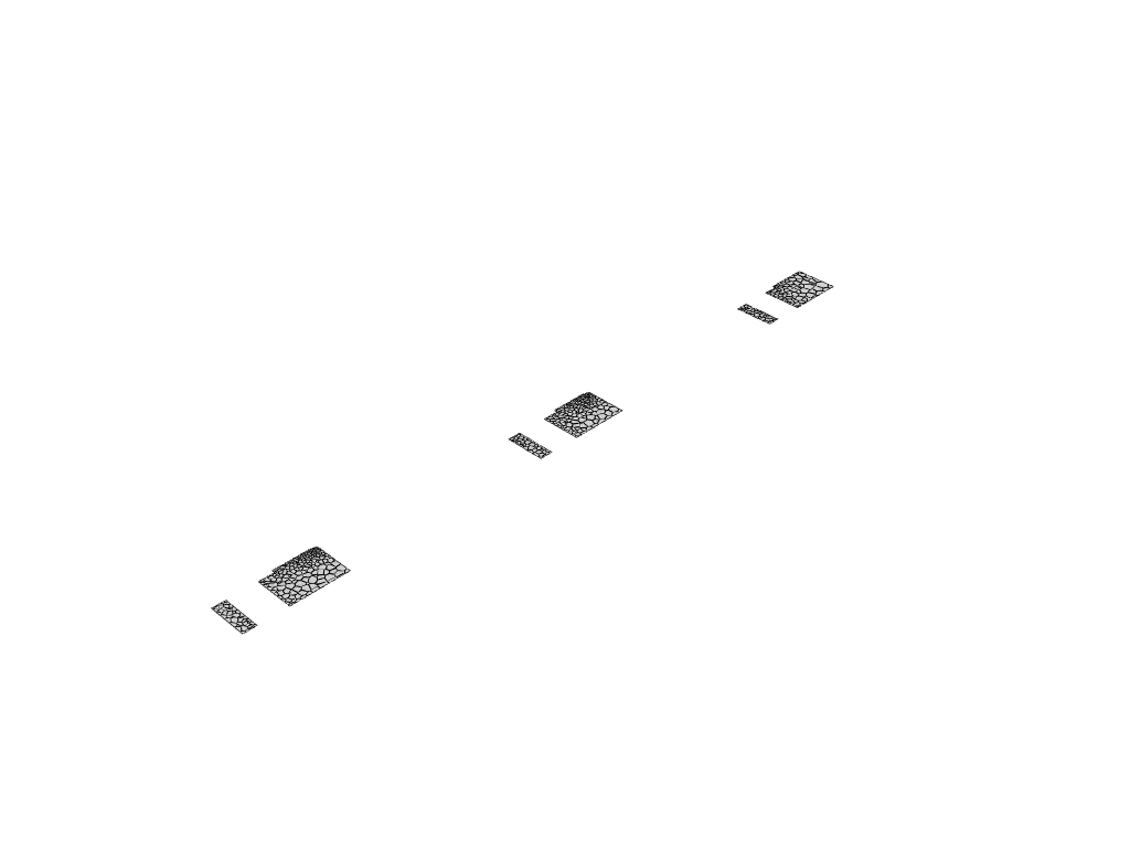
Create plane-surface XY plane

surf_xy_plane = graphics.Surfaces["xy-plane"]
surf_xy_plane.definition.type = "plane-surface"
plane_surface_xy = surf_xy_plane.definition.plane_surface
plane_surface_xy.z = -0.0441921
surf_xy_plane.display("window-3")

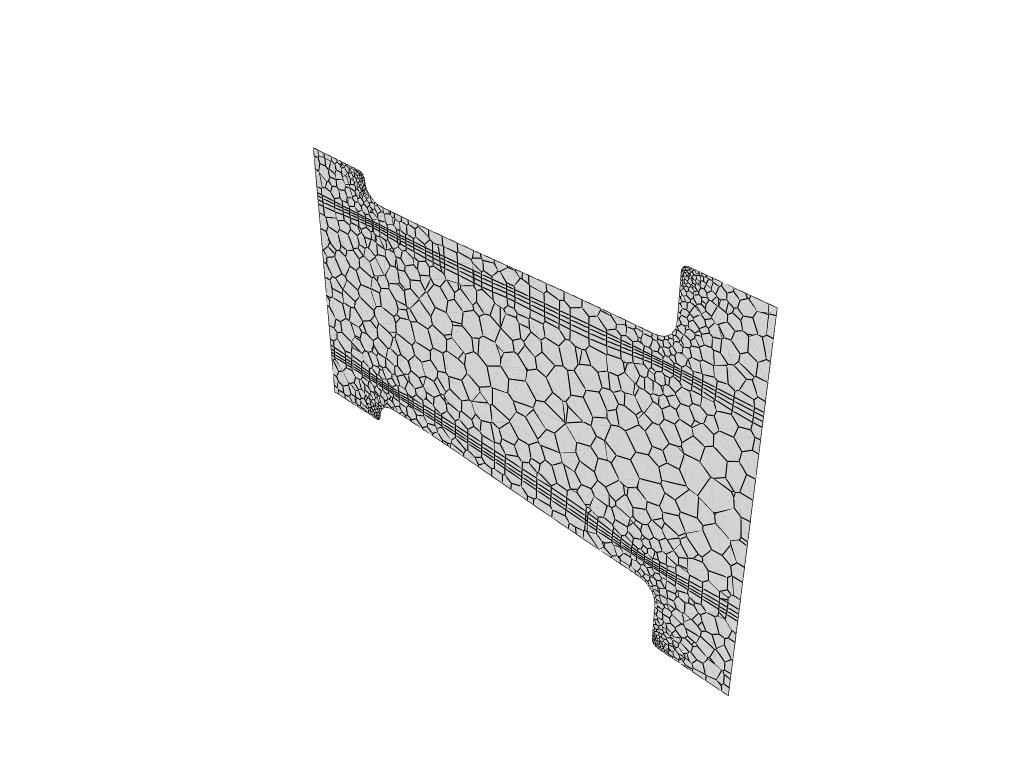
Create plane-surface YZ plane

surf_yz_plane = graphics.Surfaces["yz-plane"]
surf_yz_plane.definition.type = "plane-surface"
plane_surface_yz = surf_yz_plane.definition.plane_surface
plane_surface_yz.x = -0.174628
surf_yz_plane.display("window-4")

Create plane-surface ZX plane

surf_zx_plane = graphics.Surfaces["zx-plane"]
surf_zx_plane.definition.type = "plane-surface"
plane_surface_zx = surf_zx_plane.definition.plane_surface
plane_surface_zx.y = -0.0627297
surf_zx_plane.display("window-5")

Create iso-surface on the outlet plane

surf_outlet_plane = graphics.Surfaces["outlet-plane"]
surf_outlet_plane.definition.type = "iso-surface"
iso_surf1 = surf_outlet_plane.definition.iso_surface
iso_surf1.field = "y-coordinate"
iso_surf1.iso_value = -0.125017
surf_outlet_plane.display("window-3")

Create iso-surface on the mid-plane

surf_mid_plane_x = graphics.Surfaces["mid-plane-x"]
surf_mid_plane_x.definition.type = "iso-surface"
iso_surf2 = surf_mid_plane_x.definition.iso_surface
iso_surf2.field = "x-coordinate"
iso_surf2.iso_value = -0.174
surf_mid_plane_x.display("window-4")

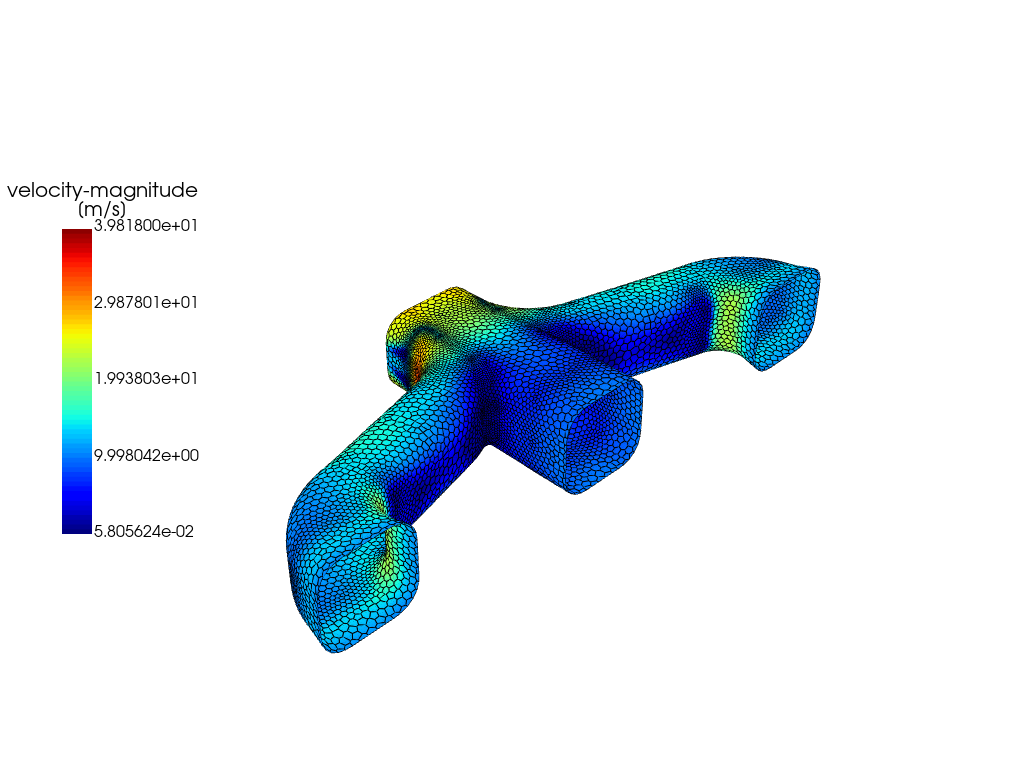
Create iso-surface using the velocity magnitude

surf_vel_contour = graphics.Surfaces["surf-vel-contour"]
surf_vel_contour.definition.type = "iso-surface"
iso_surf3 = surf_vel_contour.definition.iso_surface
iso_surf3.field = "velocity-magnitude"
iso_surf3.rendering = "contour"
iso_surf3.iso_value = 0.0
surf_vel_contour.display("window-5")

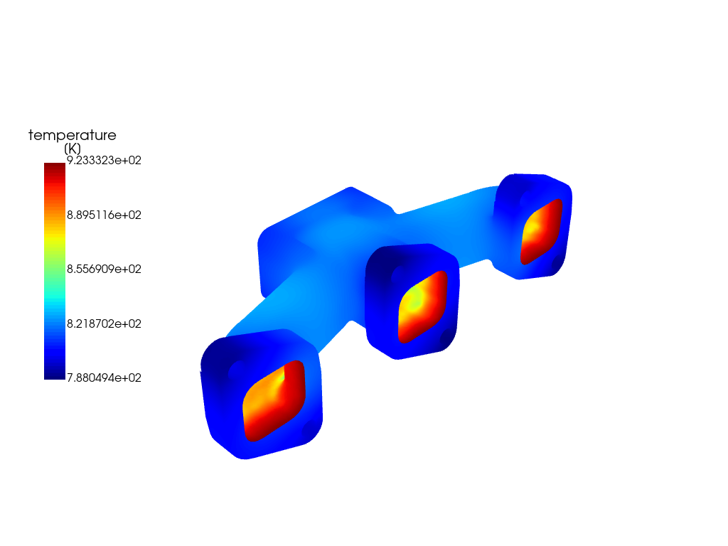
Temperature contour on the mid-plane and the outlet

temperature_contour = graphics.Contours["contour-temperature"]
temperature_contour.field = "temperature"
temperature_contour.surfaces_list = ["mid-plane-x", "outlet-plane"]
temperature_contour.display("window-6")

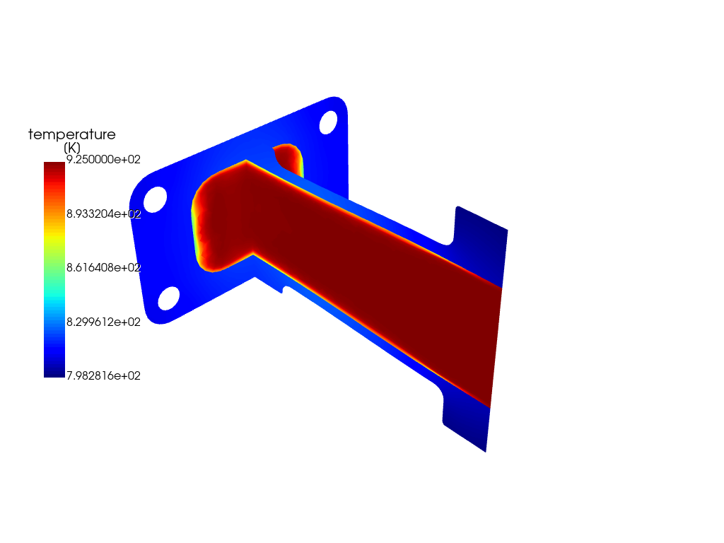
Contour plot of temperature on the manifold

temperature_contour_manifold = graphics.Contours["contour-temperature-manifold"]
temperature_contour_manifold.field = "temperature"
temperature_contour_manifold.surfaces_list = [
    "in1",
    "in2",
    "in3",
    "out1",
    "solid_up:1",
    "solid_up:1:830",
]
temperature_contour_manifold.display("window-7")

Vector on a predefined surface

velocity_vector = graphics.Vectors["velocity-vector"]
velocity_vector.surfaces_list = ["solid_up:1:830"]
velocity_vector.scale = 2
velocity_vector.display("window-8")

Start the Plot Object for the session

plots_session_1 = Plots(session)

Create a default XY-Plot

xy_plot = plots_session_1.XYPlots["xy-plot"]

Set the surface on which the plot is plotted and the Y-axis function

xy_plot.surfaces_list = ["outlet"]
xy_plot.y_axis_function = "temperature"

Plot the created XY-Plot

xy_plot.plot("window-9")

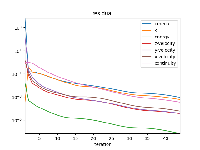
Plot residual

matplotlib_plots1 = Plots(session)
residual = matplotlib_plots1.Monitors["residual"]
residual.monitor_set_name = "residual"
residual.plot("window-10")

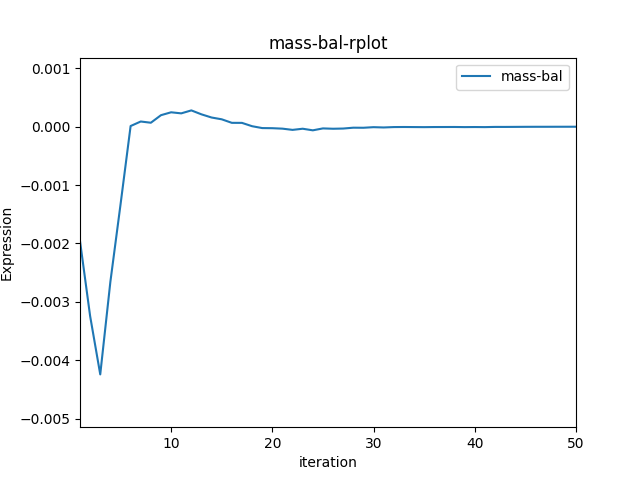
Solve and Plot Solution Monitors.

session.solver.tui.solve.initialize.hyb_initialization()
session.solver.tui.solve.set.number_of_iterations(50)
session.solver.tui.solve.iterate()
matplotlib_plots1 = Plots(session)
mass_bal_rplot = matplotlib_plots1.Monitors["mass-bal-rplot"]
mass_bal_rplot.monitor_set_name = "mass-bal-rplot"
mass_bal_rplot.plot("window-11")

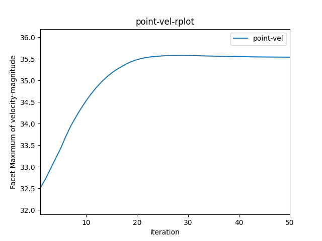
matplotlib_plots1 = Plots(session)
point_vel_rplot = matplotlib_plots1.Monitors["point-vel-rplot"]
point_vel_rplot.monitor_set_name = "point-vel-rplot"
point_vel_rplot.plot("window-12")

• 
• 

Close Fluent

session.exit()