Postprocessing using PyVista and Matplotlib

This example uses PyVista and Matplotlib to demonstrate PyFluent postprocessing capabilities. The 3D model in this example is an exhaust manifold that has high temperature flows passing through it. The flow through the manifold is turbulent and involves conjugate heat transfer.

Perform required imports

Perform required imports and set the configuration.

import ansys.fluent.core as pyfluent
from ansys.fluent.core import examples

from ansys.fluent.visualization import set_config
from ansys.fluent.visualization.matplotlib import Plots
from ansys.fluent.visualization.pyvista import Graphics

set_config(blocking=True, set_view_on_display="isometric")

Download files and launch Fluent

Download the case and data files and launch Fluent as a service in solver mode with double precision and two processors. Read in the case and data files.

import_case = examples.download_file(
    filename="exhaust_system.cas.h5", directory="pyfluent/exhaust_system"
)

import_data = examples.download_file(
    filename="exhaust_system.dat.h5", directory="pyfluent/exhaust_system"
)

solver_session = pyfluent.launch_fluent(
    precision="double", processor_count=2, start_transcript=False, mode="solver"
)

solver_session.tui.file.read_case(import_case)
solver_session.tui.file.read_data(import_data)

Get graphics object

Get the graphics object.

graphics = Graphics(session=solver_session)

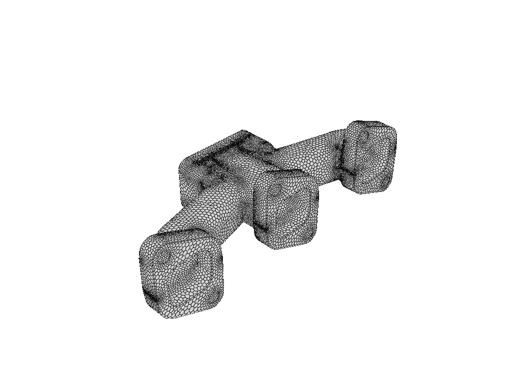
Create graphics object for mesh display

Create a graphics object for the mesh display.

mesh1 = graphics.Meshes["mesh-1"]

Show edges

Show edges on the mesh.

mesh1.show_edges = True

Get surfaces list

Get the surfaccase list.

mesh1.surfaces_list = [
    "in1",
    "in2",
    "in3",
    "out1",
    "solid_up:1",
    "solid_up:1:830",
    "solid_up:1:830-shadow",
]
mesh1.display("window-1")

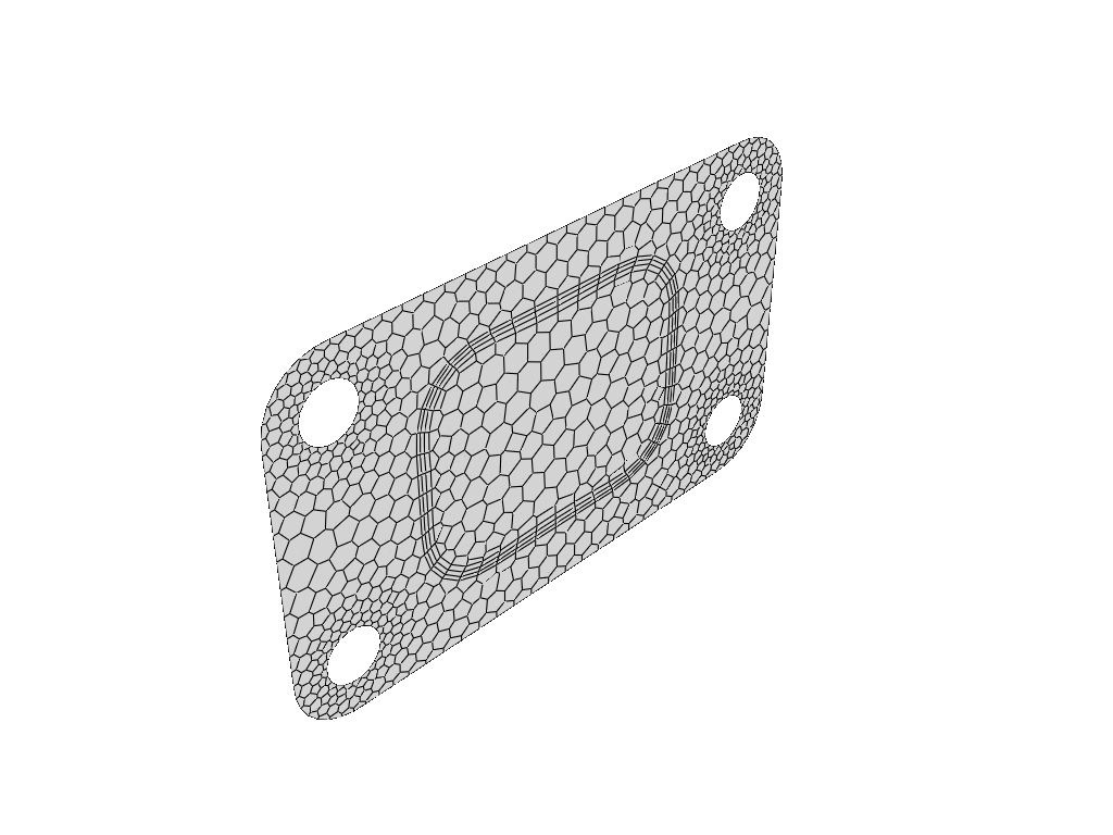
Hide edges and display again

Hide the edges and display again.

mesh1.show_edges = False
mesh1.display("window-2")

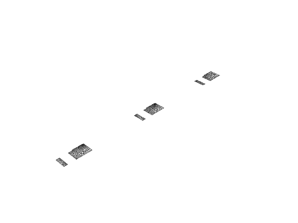
Create plane-surface XY plane

Create a plane-surface XY plane.

surf_xy_plane = graphics.Surfaces["xy-plane"]
surf_xy_plane.definition.type = "plane-surface"
plane_surface_xy = surf_xy_plane.definition.plane_surface
plane_surface_xy.z = -0.0441921
surf_xy_plane.display("window-3")

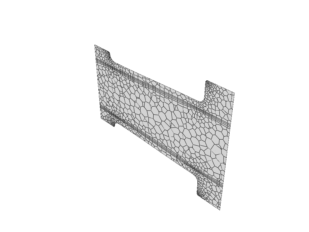
Create plane-surface YZ plane

Create a plane-surface YZ plane.

surf_yz_plane = graphics.Surfaces["yz-plane"]
surf_yz_plane.definition.type = "plane-surface"
plane_surface_yz = surf_yz_plane.definition.plane_surface
plane_surface_yz.x = -0.174628
surf_yz_plane.display("window-4")

Create plane-surface ZX plane

Create a plane-surface ZX plane.

surf_zx_plane = graphics.Surfaces["zx-plane"]
surf_zx_plane.definition.type = "plane-surface"
plane_surface_zx = surf_zx_plane.definition.plane_surface
plane_surface_zx.y = -0.0627297
surf_zx_plane.display("window-5")

Create iso-surface on outlet plane

Create an iso-surface on the outlet plane.

surf_outlet_plane = graphics.Surfaces["outlet-plane"]
surf_outlet_plane.definition.type = "iso-surface"
iso_surf1 = surf_outlet_plane.definition.iso_surface
iso_surf1.field = "y-coordinate"
iso_surf1.iso_value = -0.125017
surf_outlet_plane.display("window-3")

Create iso-surface on mid-plane

Create an iso-surface on the mid-plane.

surf_mid_plane_x = graphics.Surfaces["mid-plane-x"]
surf_mid_plane_x.definition.type = "iso-surface"
iso_surf2 = surf_mid_plane_x.definition.iso_surface
iso_surf2.field = "x-coordinate"
iso_surf2.iso_value = -0.174
surf_mid_plane_x.display("window-4")

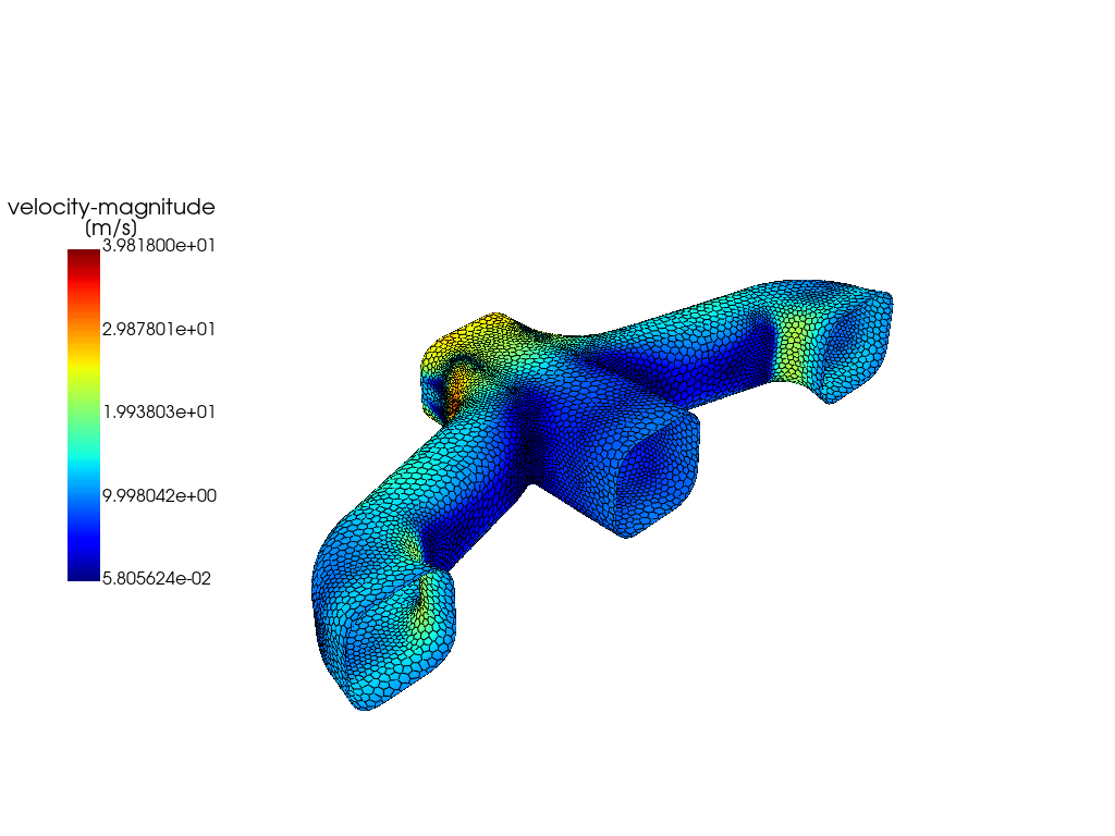
Create iso-surface using velocity magnitude

Create an iso-surface using the velocity magnitude.

surf_vel_contour = graphics.Surfaces["surf-vel-contour"]
surf_vel_contour.definition.type = "iso-surface"
iso_surf3 = surf_vel_contour.definition.iso_surface
iso_surf3.field = "velocity-magnitude"
iso_surf3.rendering = "contour"
iso_surf3.iso_value = 0.0
surf_vel_contour.display("window-5")

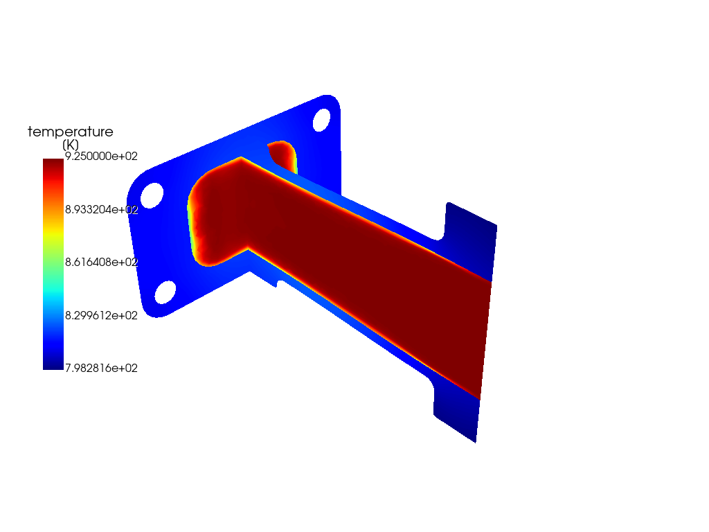
Create temperature contour on mid-plane and outlet

Create a temperature contour on the mid-plane and the outlet.

temperature_contour = graphics.Contours["contour-temperature"]
temperature_contour.field = "temperature"
temperature_contour.surfaces_list = ["mid-plane-x", "outlet-plane"]
temperature_contour.display("window-6")

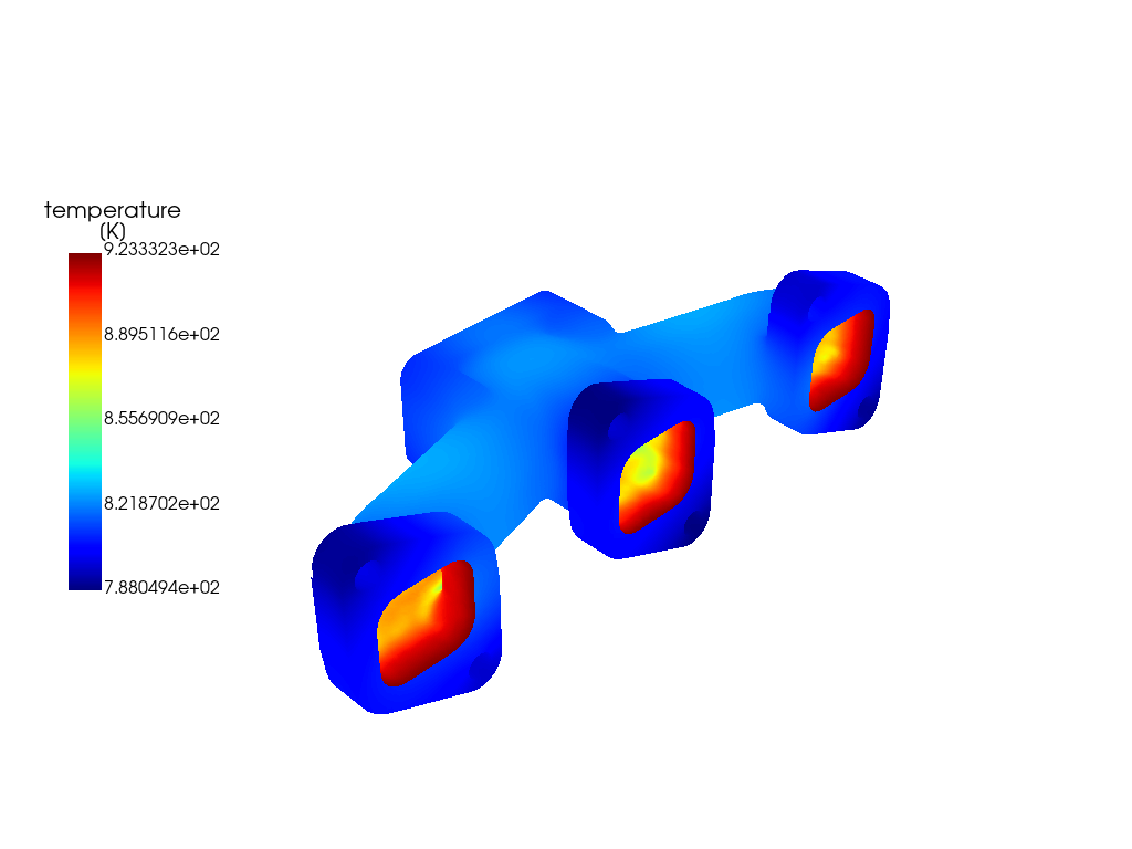
Create contour plot of temperature on manifold

Create a contour plot of the temperature on the manifold.

temperature_contour_manifold = graphics.Contours["contour-temperature-manifold"]
temperature_contour_manifold.field = "temperature"
temperature_contour_manifold.surfaces_list = [
    "in1",
    "in2",
    "in3",
    "out1",
    "solid_up:1",
    "solid_up:1:830",
]
temperature_contour_manifold.display("window-7")

Create vector

Create a vector on a predefined surface.

velocity_vector = graphics.Vectors["velocity-vector"]
velocity_vector.field = "pressure"
velocity_vector.surfaces_list = ["solid_up:1:830"]
velocity_vector.scale = 2
velocity_vector.display("window-8")

Create Pathlines

Create a pathlines on a predefined surface.

pathlines = graphics.Pathlines["pathlines"]
pathlines.field = "velocity-magnitude"
pathlines.surfaces_list = ["inlet", "inlet1", "inlet2"]
# pathlines.display("window-9")

Create plot object

Create the plot object for the session.

plots_session_1 = Plots(solver_session)

Create XY plot

Create the default XY plot.

xy_plot = plots_session_1.XYPlots["xy-plot"]

Set plot surface and Y-axis function

Set the surface on which to generate the plot and the Y-axis function.

xy_plot.surfaces_list = ["outlet"]
xy_plot.y_axis_function = "temperature"

Display XY plot

Display the generated XY plot.

xy_plot.plot("window-9")

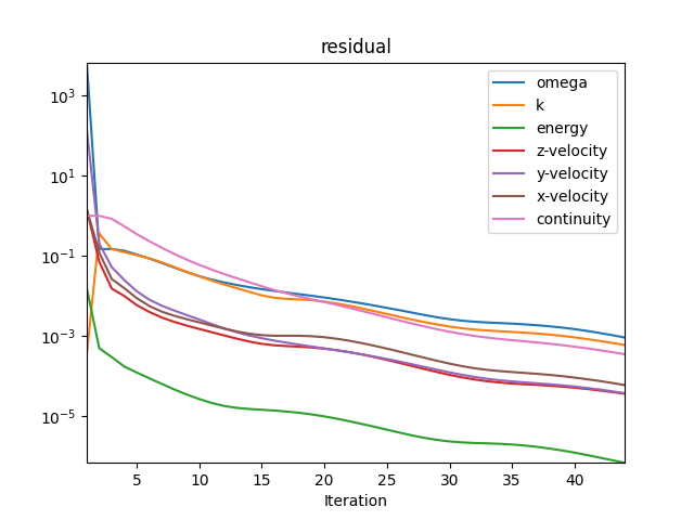
Create residual plot

Create and display the residual plot.

matplotlib_plots1 = Plots(solver_session)
residual = matplotlib_plots1.Monitors["residual"]
residual.monitor_set_name = "residual"
residual.plot("window-10")

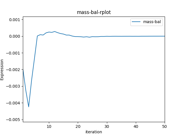
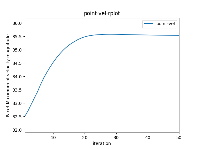
Solve and plot solution monitors

Solve and plot solution monitors.

solver_session.tui.solve.initialize.hyb_initialization()
solver_session.tui.solve.set.number_of_iterations(50)
solver_session.tui.solve.iterate()
matplotlib_plots1 = Plots(solver_session)
mass_bal_rplot = matplotlib_plots1.Monitors["mass-bal-rplot"]
mass_bal_rplot.monitor_set_name = "mass-bal-rplot"
mass_bal_rplot.plot("window-11")

matplotlib_plots1 = Plots(solver_session)
point_vel_rplot = matplotlib_plots1.Monitors["point-vel-rplot"]
point_vel_rplot.monitor_set_name = "point-vel-rplot"
point_vel_rplot.plot("window-12")

• 
• 

Close Fluent

Close Fluent.

solver_session.exit()