Enhanced Postprocessing

This updated example demonstrates postprocessing capabilities in PyFluent using an object-oriented approach, providing a more user-friendly interface and improved flexibility. The 3D model used in this example is an exhaust manifold, where high-temperature turbulent flows are analyzed in a conjugate heat transfer scenario.

Key Improvements:

Object-Oriented Design: The code has been modularized into classes and methods, enhancing maintainability and reusability.

Interactive User Interface: The user interface now allows seamless interaction, enabling users to control and customize postprocessing parameters.

Enhanced Plot Interaction: Users have greater freedom to interact with the plots, such as adding and super-imposing multiple plots, and toggling data views, enhancing the visualization experience.

This example utilizes PyVista for 3D visualization and for 2D data plotting. The new design provides a streamlined workflow for exploring and analyzing the temperature and flow characteristics in the exhaust manifold.

Run the following in command prompt to execute this file: exec(open(“updated_post_processing_example.py”).read())

Perform required imports

Perform required imports and set the configuration.

import ansys.fluent.core as pyfluent
from ansys.fluent.core import examples
from ansys.fluent.core.solver import (
    PressureOutlets,
    VelocityInlets,
    WallBoundaries,
    WallBoundary,
    using,
)
from ansys.units import VariableCatalog

from ansys.fluent.visualization import (
    Contour,
    GraphicsWindow,
    IsoSurface,
    Mesh,
    Monitor,
    Pathline,
    PlaneSurface,
    Vector,
    XYPlot,
    config,
)

pyfluent.CONTAINER_MOUNT_PATH = pyfluent.EXAMPLES_PATH

config.interactive = False
config.view = "isometric"

Download files and launch Fluent

Download the case and data files and launch Fluent as a service in solver mode with double precision and two processors. Read in the case and data files.

import_case = examples.download_file(
    file_name="exhaust_system.cas.h5", directory="pyfluent/exhaust_system"
)

import_data = examples.download_file(
    file_name="exhaust_system.dat.h5", directory="pyfluent/exhaust_system"
)

solver_session = pyfluent.launch_fluent(
    precision=pyfluent.Precision.DOUBLE,
    processor_count=2,
    start_transcript=False,
    mode=pyfluent.FluentMode.SOLVER,
)

solver_session.settings.file.read_case(file_name=import_case)
solver_session.settings.file.read_data(file_name=import_data)

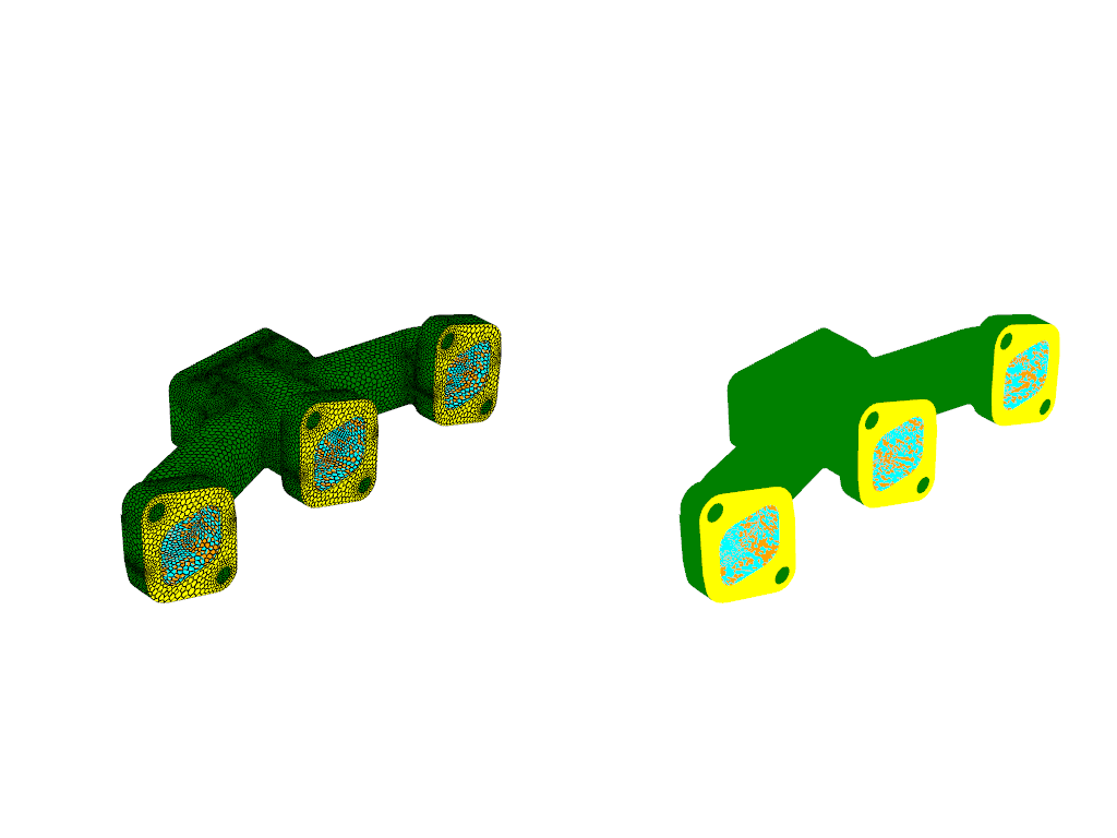
with using(solver_session):

    # Create a graphics object for the mesh display.
    graphics_window = GraphicsWindow()

    mesh = Mesh(show_edges=True, surfaces=WallBoundaries())
    graphics_window.add_graphics(mesh, position=(0, 0))

    mesh = Mesh(surfaces=WallBoundaries())
    graphics_window.add_graphics(mesh, position=(0, 1))

    graphics_window.show()

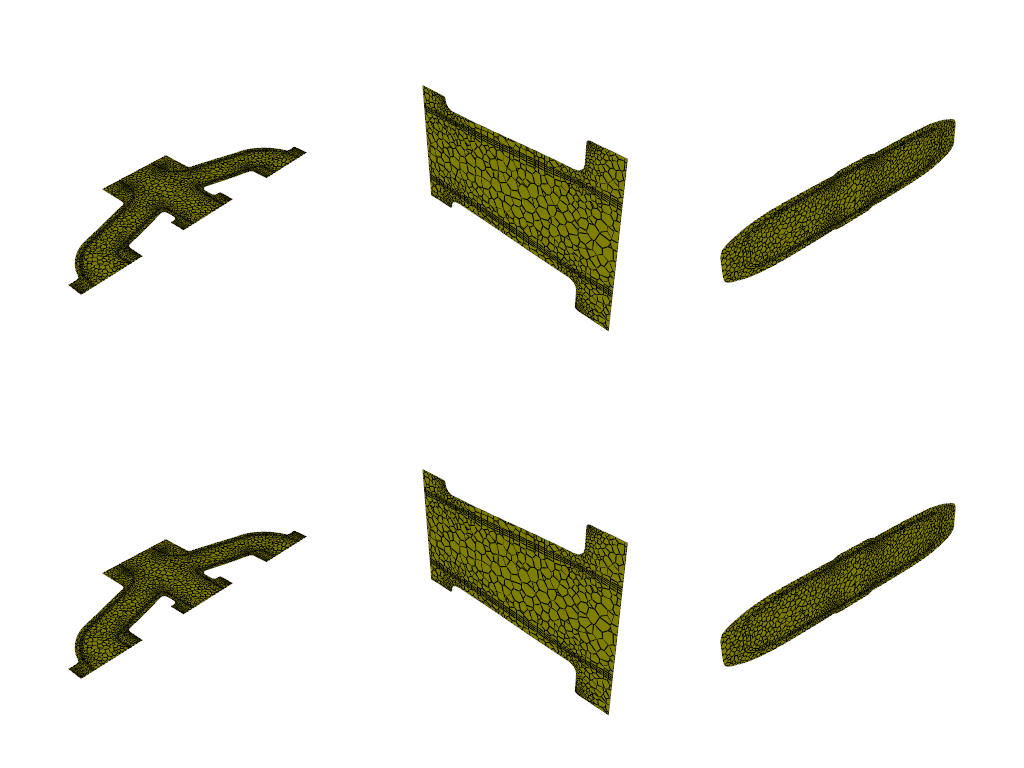
    # Create XY, YZ, ZX and an arbitrary plane-surface objects
    # from point and normal and display.
    graphics_window = GraphicsWindow()

    surf_xy_plane = PlaneSurface.create_from_point_and_normal(
        point=[0.0, 0.0, -0.0441921], normal=[0.0, 0.0, 1.0]
    )
    graphics_window.add_graphics(surf_xy_plane, position=(0, 0))

    surf_yz_plane = PlaneSurface.create_from_point_and_normal(
        point=[-0.174628, 0.0, 0.0], normal=[1.0, 0.0, 0.0]
    )
    graphics_window.add_graphics(surf_yz_plane, position=(0, 1))

    surf_zx_plane = PlaneSurface.create_from_point_and_normal(
        point=[0.0, -0.0627297, 0.0], normal=[0.0, 1.0, 0.0]
    )
    graphics_window.add_graphics(surf_zx_plane, position=(0, 2))

    # Create XY, YZ and ZX plane-surface objects and display.
    surf_xy_plane = PlaneSurface.create_xy_plane(z=-0.0441921)
    graphics_window.add_graphics(surf_xy_plane, position=(1, 0))

    surf_yz_plane = PlaneSurface.create_yz_plane(x=-0.174628)
    graphics_window.add_graphics(surf_yz_plane, position=(1, 1))

    surf_zx_plane = PlaneSurface.create_zx_plane(y=-0.0627297)
    graphics_window.add_graphics(surf_zx_plane, position=(1, 2))

    graphics_window.show()

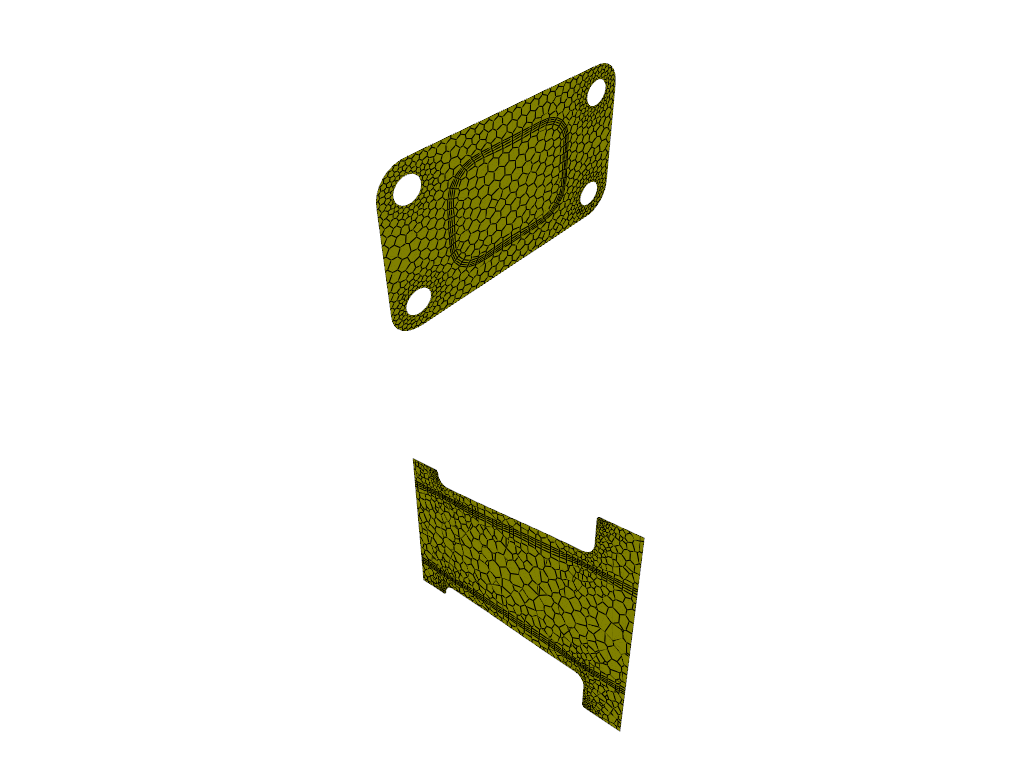
    # Create an iso-surface on the outlet and mid-plane.
    graphics_window = GraphicsWindow()

    surf_outlet_plane = IsoSurface(field="y-coordinate", iso_value=-0.125017)
    graphics_window.add_graphics(surf_outlet_plane, position=(0, 0))

    surf_mid_plane_x = IsoSurface(field="x-coordinate", iso_value=-0.174)
    graphics_window.add_graphics(surf_mid_plane_x, position=(1, 0))

    graphics_window.show()

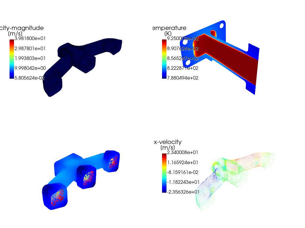
    # Create an iso-surface using the velocity magnitude, a temperature contour
    # on the mid-plane and the outlet, a contour plot of the temperature on the
    # manifold and a vector on a predefined surface.
    graphics_window = GraphicsWindow()

    surf_vel_contour = IsoSurface(
        field=VariableCatalog.VELOCITY_MAGNITUDE, rendering="contour", iso_value=0.0
    )
    graphics_window.add_graphics(surf_vel_contour)

    temperature_contour = Contour(
        field=VariableCatalog.TEMPERATURE,
        surfaces=[surf_mid_plane_x.name, surf_outlet_plane.name],
    )
    graphics_window.add_graphics(temperature_contour, position=(0, 1))

    temperature_contour_manifold = Contour(
        field=VariableCatalog.TEMPERATURE, surfaces=WallBoundaries()
    )
    graphics_window.add_graphics(temperature_contour_manifold, position=(1, 0))

    velocity_vector = Vector(
        field=VariableCatalog.VELOCITY_X,
        surfaces=[WallBoundary(name="solid_up:1:830")],
        scale=20,
    )
    graphics_window.add_graphics(velocity_vector, position=(1, 1))

    graphics_window.show()

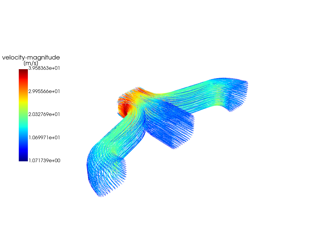
    # Create a pathlines on a predefined surface.
    graphics_window = GraphicsWindow()

    pathlines = Pathline(
        field=VariableCatalog.VELOCITY_MAGNITUDE, surfaces=VelocityInlets()
    )
    graphics_window.add_graphics(pathlines)

    graphics_window.show()

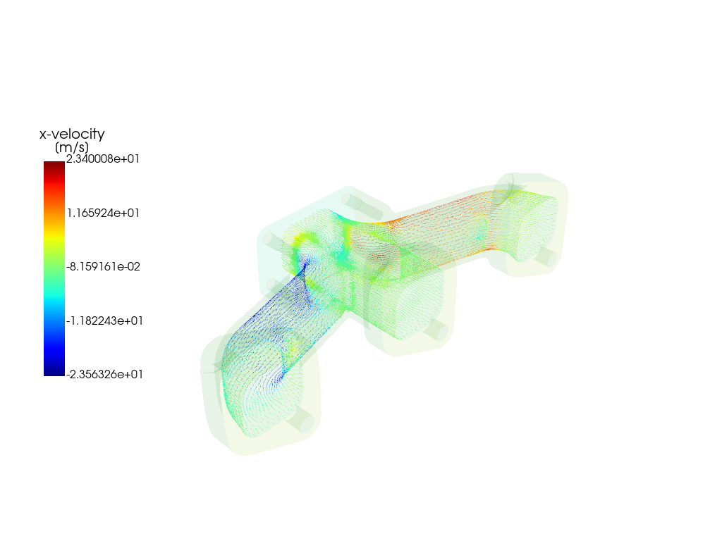
    # Create a combined mesh and vector plot by varying opacity.
    graphics_window = GraphicsWindow()

    graphics_window.add_graphics(mesh, opacity=0.05)
    graphics_window.add_graphics(velocity_vector)

    graphics_window.show()

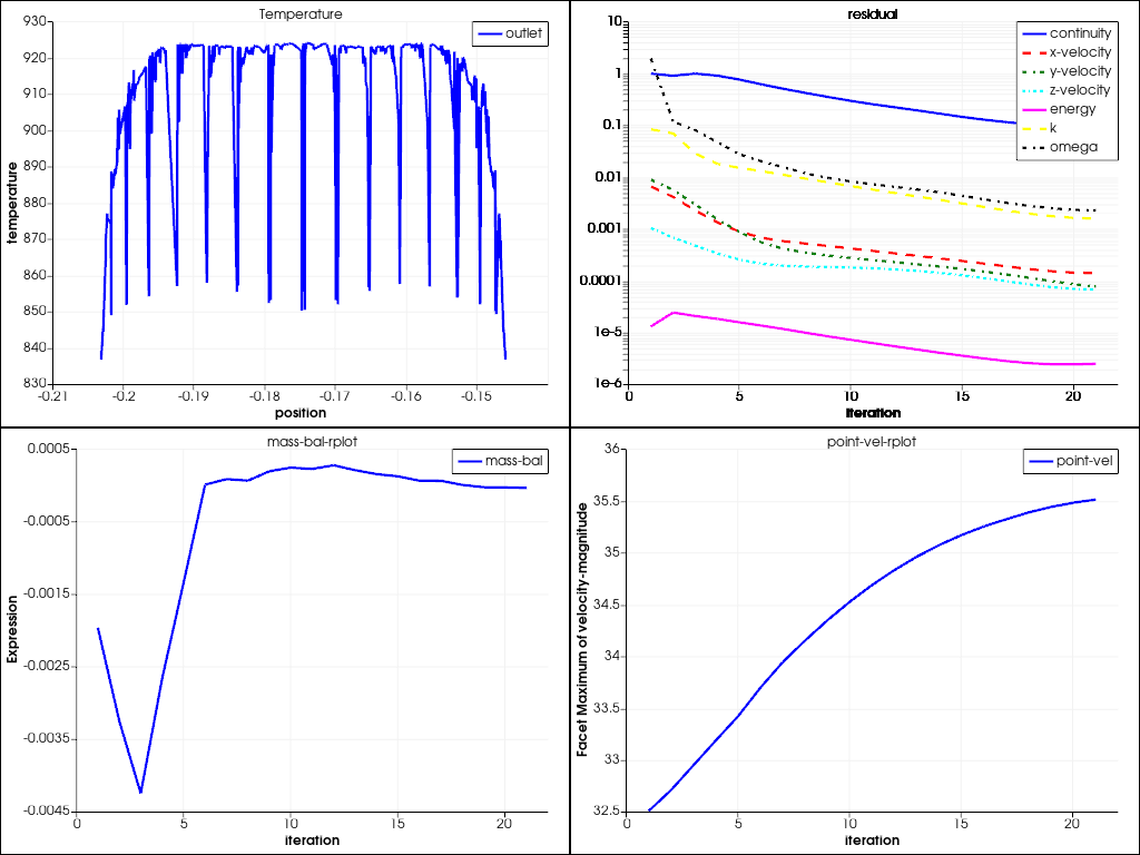
    # Create and display XY plot, residual plot and solve and plot solution monitors.
    plot_window = GraphicsWindow()

    xy_plot_object = XYPlot(
        surfaces=PressureOutlets(), y_axis_function=VariableCatalog.TEMPERATURE
    )
    plot_window.add_plot(xy_plot_object, position=(0, 0), title="Temperature")

    residual = Monitor(monitor_set_name="residual")
    plot_window.add_plot(residual, position=(0, 1))

    solver_session.solution.initialization.hybrid_initialize()
    solver_session.solution.run_calculation.iterate(iter_count=50)

    mass_bal_rplot = Monitor(monitor_set_name="mass-bal-rplot")
    plot_window.add_plot(mass_bal_rplot, position=(1, 0))

    point_vel_rplot = Monitor(monitor_set_name="point-vel-rplot")
    plot_window.add_plot(point_vel_rplot, position=(1, 1))

    plot_window.show()

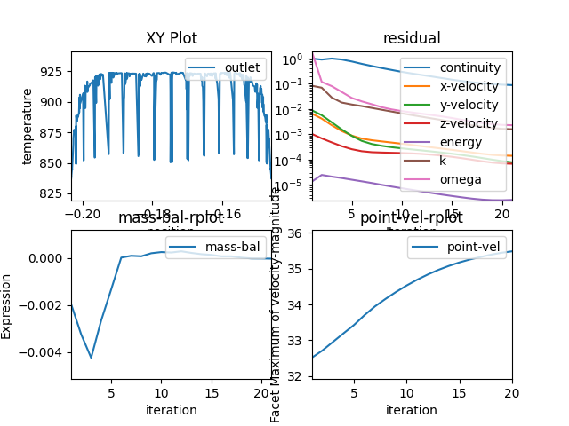
    plot_window.renderer = "matplotlib"
    plot_window.show()

• 
• 
• 
• 
• 
• 
•