Post-processing using Pyvista and Matplotlib

This example shows how to use PyFluent’s post-processing tools to visualize Fluent results in both 3D and 2D. It demonstrates a typical workflow for exploring simulation data—such as temperature and velocity fields—using Pyvista for interactive 3D graphics and Matplotlib for standard 2D plots.

The model used here is an exhaust manifold, but the techniques apply to any Fluent simulation.

What this example demonstrates

• 3D Visualization with Pyvista: Display meshes, surfaces, iso-surfaces, contours, vectors, and pathlines to understand spatial flow behavior.

• 2D Plotting with Matplotlib: Create XY plots such as temperature or velocity profiles, monitor quantities, and compare numerical trends.

• Simple, Practical Workflow: Shows how to load results, create common visualization objects, adjust display settings, and interact with the scene — all with clear, straightforward commands.

• Unified Post-Processing Interface: Combines 3D and 2D visualization tools so users can inspect their results from multiple perspectives within a single, consistent workflow.

This example provides a concise starting point for analyzing Fluent simulations visually, without requiring knowledge of internal APIs or implementation details.

Perform required imports

Perform required imports and set the configuration.

import ansys.fluent.core as pyfluent
from ansys.fluent.core import examples
from ansys.units import VariableCatalog

from ansys.fluent.visualization import (
    Contour,
    GraphicsWindow,
    Mesh,
    Monitor,
    Pathline,
    Surface,
    Vector,
    XYPlot,
    config,
)

pyfluent.CONTAINER_MOUNT_PATH = pyfluent.EXAMPLES_PATH

config.interactive = False
config.view = "isometric"

Download files and launch Fluent

Download the case and data files and launch Fluent as a service in solver mode with double precision and two processors. Read in the case and data files.

import_case = examples.download_file(
    file_name="exhaust_system.cas.h5", directory="pyfluent/exhaust_system"
)

import_data = examples.download_file(
    file_name="exhaust_system.dat.h5", directory="pyfluent/exhaust_system"
)

solver_session = pyfluent.launch_fluent(
    precision=pyfluent.Precision.DOUBLE,
    processor_count=2,
    start_transcript=False,
    mode=pyfluent.FluentMode.SOLVER,
)

solver_session.settings.file.read_case(file_name=import_case)
solver_session.settings.file.read_data(file_name=import_data)

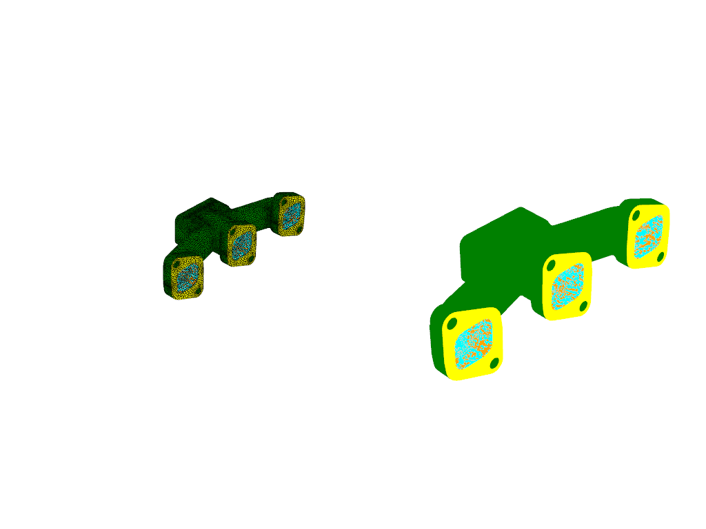
Create graphics object for mesh display

Create a graphics object for the mesh display.

mesh_surfaces_list = [
    "in1",
    "in2",
    "in3",
    "out1",
    "solid_up:1",
    "solid_up:1:830",
    "solid_up:1:830-shadow",
]
mesh = Mesh(solver=solver_session, show_edges=True, surfaces=mesh_surfaces_list)
graphics_window = GraphicsWindow()
graphics_window.add_graphics(mesh, position=(0, 0))

mesh = Mesh(solver=solver_session, surfaces=mesh_surfaces_list)
graphics_window.add_graphics(mesh, position=(0, 1))
graphics_window.show()

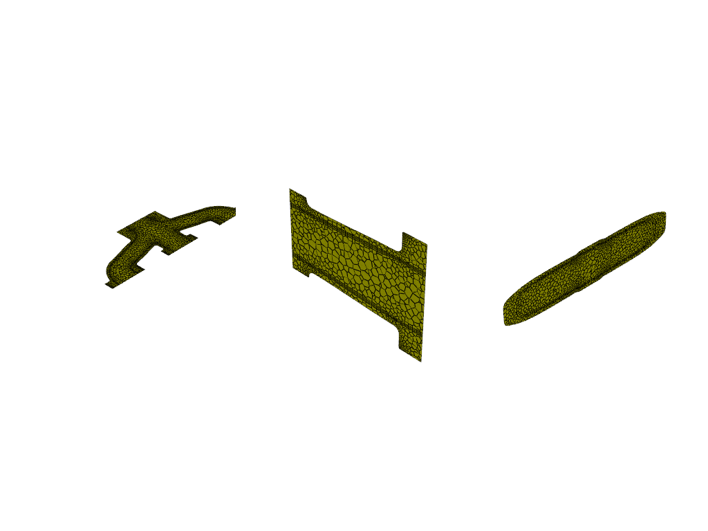
Create plane-surface XY plane

Create a plane-surface XY plane.

surf_xy_plane = Surface(
    solver=solver_session,
    type="plane-surface",
    creation_method="xy-plane",
    z=-0.0441921,
)
graphics_window = GraphicsWindow()
graphics_window.add_graphics(surf_xy_plane, position=(0, 0))

Create plane-surface YZ plane

Create a plane-surface YZ plane.

surf_yz_plane = Surface(
    solver=solver_session, type="plane-surface", creation_method="yz-plane", x=-0.174628
)
graphics_window.add_graphics(surf_yz_plane, position=(0, 1))

Create plane-surface ZX plane

Create a plane-surface ZX plane.

surf_zx_plane = Surface(
    solver=solver_session,
    type="plane-surface",
    creation_method="zx-plane",
    y=-0.0627297,
)
graphics_window.add_graphics(surf_zx_plane, position=(0, 2))
graphics_window.show()

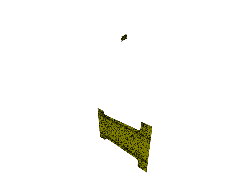
Create iso-surface on outlet plane

Create an iso-surface on the outlet plane.

surf_outlet_plane = Surface(solver=solver_session, type="iso-surface")
surf_outlet_plane.field = "y-coordinate"
surf_outlet_plane.iso_value = -0.125017
graphics_window = GraphicsWindow()
graphics_window.add_graphics(surf_outlet_plane, position=(0, 0))

Create iso-surface on mid-plane

Create an iso-surface on the mid-plane.

surf_mid_plane_x = Surface(
    solver=solver_session, type="iso-surface", field="x-coordinate", iso_value=-0.174
)
graphics_window.add_graphics(surf_mid_plane_x, position=(1, 0))
graphics_window.show()

Create iso-surface using velocity magnitude

Create an iso-surface using the velocity magnitude.

surf_vel_contour = Surface(
    solver=solver_session,
    type="iso-surface",
    field="velocity-magnitude",
    rendering="contour",
    iso_value=0.0,
)
graphics_window = GraphicsWindow()
graphics_window.add_graphics(surf_vel_contour, position=(0, 0))

Create temperature contour on mid-plane and outlet

Create a temperature contour on the mid-plane and the outlet.

temperature_contour = Contour(
    solver=solver_session,
    field="temperature",
    surfaces=[surf_mid_plane_x.name, surf_outlet_plane.name],
)
graphics_window.add_graphics(temperature_contour, position=(0, 1))

Create contour plot of temperature on manifold

Create a contour plot of the temperature on the manifold.

cont_surfaces_list = [
    "in1",
    "in2",
    "in3",
    "out1",
    "solid_up:1",
    "solid_up:1:830",
]
temperature_contour_manifold = Contour(
    solver=solver_session,
    field=VariableCatalog.TEMPERATURE,
    surfaces=cont_surfaces_list,
)
graphics_window.add_graphics(temperature_contour_manifold, position=(1, 0))

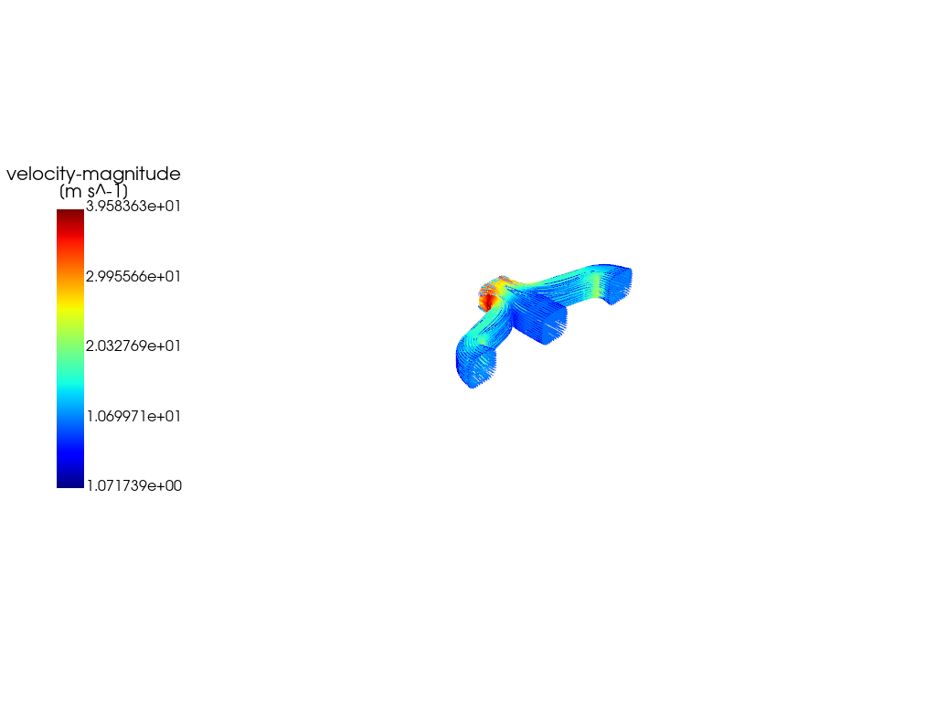
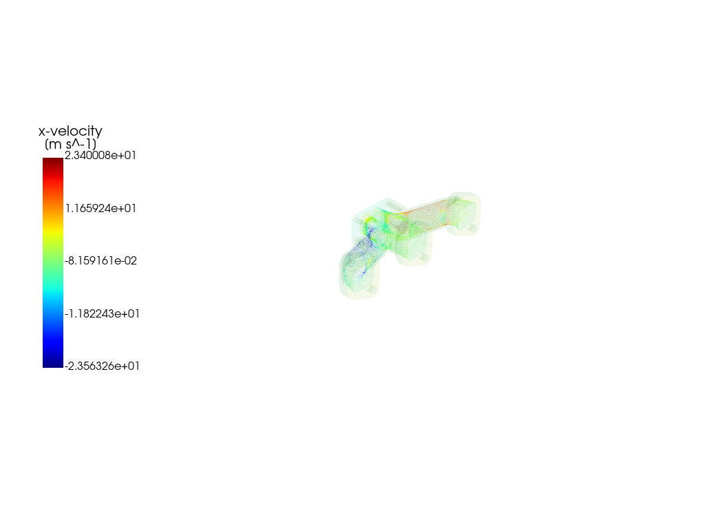
Create vector

Create a vector on a predefined surface.

velocity_vector = Vector(
    solver=solver_session,
    field="velocity",
    color_by="x-velocity",
    surfaces=["solid_up:1:830"],
    scale=20,
)
graphics_window.add_graphics(velocity_vector, position=(1, 1))
graphics_window.show()

Create Pathlines

Create a pathlines on a predefined surface.

pathlines = Pathline(
    solver=solver_session,
    field="velocity-magnitude",
    surfaces=["inlet", "inlet1", "inlet2"],
)

graphics_window = GraphicsWindow()
graphics_window.add_graphics(pathlines)
graphics_window.show()

graphics_window = GraphicsWindow()
graphics_window.add_graphics(mesh, opacity=0.05)
graphics_window.add_graphics(velocity_vector)
graphics_window.show()

• 
• 

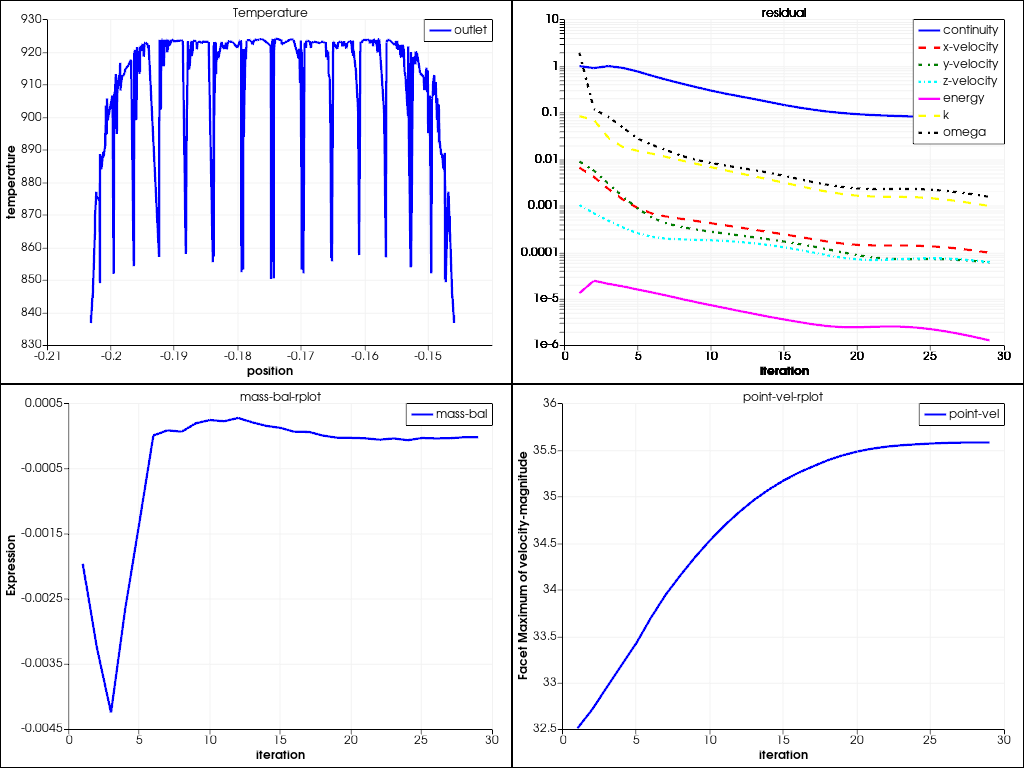
Create XY plot

Create the default XY plot.

xy_plot_object = XYPlot(
    solver=solver_session,
    surfaces=["outlet"],
    y_axis_function="temperature",
)
plot_window = GraphicsWindow()
plot_window.add_plot(xy_plot_object, position=(0, 0), title="Temperature")

Create residual plot

Create and display the residual plot.

residual = Monitor(solver=solver_session, monitor_set_name="residual")
plot_window.add_plot(residual, position=(0, 1))

Solve and plot solution monitors

Solve and plot solution monitors.

solver_session.solution.initialization.hybrid_initialize()
solver_session.solution.run_calculation.iterate(iter_count=50)

mass_bal_rplot = Monitor(solver=solver_session, monitor_set_name="mass-bal-rplot")
plot_window.add_plot(mass_bal_rplot, position=(1, 0))

point_vel_rplot = Monitor(solver=solver_session, monitor_set_name="point-vel-rplot")
plot_window.add_plot(point_vel_rplot, position=(1, 1))
plot_window.show()

Close Fluent

Close Fluent.

solver_session.exit()
del solver_session