Post-processing using Pyvista and Matplotlib plotter APIs

This example demonstrates how to perform straightforward 2D and 3D post-processing in PyFluent using the Pyvista and Matplotlib interfaces. It highlights practical tasks such as mesh display, plotting key variables, and exporting graphics for reports.

Using an exhaust manifold case, the example shows how to visualize wall boundaries, examine outlet temperature variations, and generate XY and residual plots—all through simple, scriptable API calls.

Key Features

• Mesh Visualization: View wall boundaries with optional edge highlighting for clearer geometry inspection.

• XY & Residual Plots: Generate temperature and residual plots using PyFluent’s built-in plotting interface.

• Simple Export: Save visualizations as PNG or PDF for documentation or post-processing workflows.

Overall, the example provides a clean, approachable workflow that helps users quickly extract and visualize essential solver data.

Perform required imports

Perform required imports and set the configuration.

import ansys.fluent.core as pyfluent
from ansys.fluent.core import examples
from ansys.fluent.core.solver import (
    PressureOutlets,
    WallBoundaries,
)
from ansys.units import VariableCatalog

from ansys.fluent.visualization import (
    GraphicsWindow,
    Mesh,
    Monitor,
    XYPlot,
    config,
)

pyfluent.CONTAINER_MOUNT_PATH = pyfluent.EXAMPLES_PATH

config.interactive = False
config.view = "isometric"

Download files and launch Fluent

Download the case and data files and launch Fluent as a service in solver mode with double precision and two processors. Read in the case and data files.

import_case = examples.download_file(
    file_name="exhaust_system.cas.h5", directory="pyfluent/exhaust_system"
)

import_data = examples.download_file(
    file_name="exhaust_system.dat.h5", directory="pyfluent/exhaust_system"
)

solver_session = pyfluent.launch_fluent(
    precision=pyfluent.Precision.DOUBLE,
    processor_count=2,
    start_transcript=False,
    mode=pyfluent.FluentMode.SOLVER,
)

solver_session.file.read_case_data(file_name=import_case)

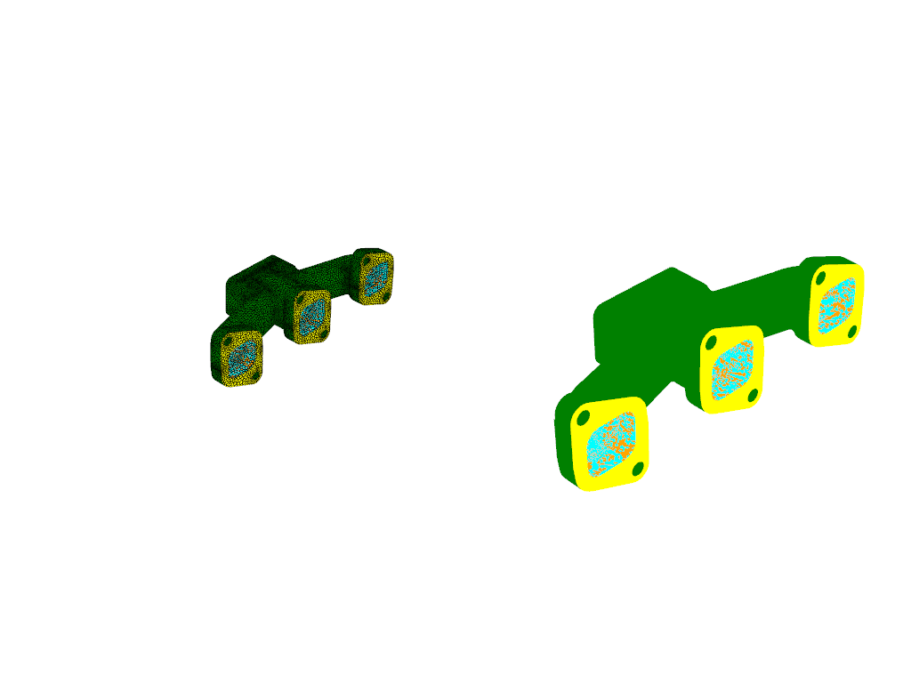
Display Mesh

Create and display the mesh for wall boundaries.

graphics_window = GraphicsWindow()

mesh = Mesh(
    solver=solver_session,
    show_edges=True,
    surfaces=WallBoundaries(settings_source=solver_session),
)
graphics_window.add_graphics(mesh, position=(0, 0))

mesh = Mesh(
    solver=solver_session, surfaces=WallBoundaries(settings_source=solver_session)
)
graphics_window.add_graphics(mesh, position=(0, 1))

graphics_window.renderer.set_background("black", top="white")
graphics_window.save_graphics("sample_mesh_image.pdf")
graphics_window.renderer.set_background("white")
graphics_window.show()

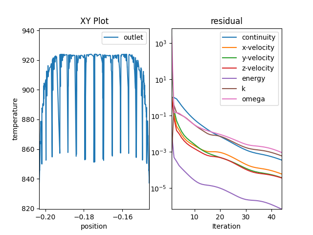
Create and Display Plots

Create and display XY and residual plots, and save them as files.

plot_window = GraphicsWindow()

xy_plot_object = XYPlot(
    solver=solver_session,
    surfaces=PressureOutlets(settings_source=solver_session),
    y_axis_function=VariableCatalog.TEMPERATURE,
)
plot_window.add_plot(xy_plot_object, position=(0, 0), title="Temperature")

residual = Monitor(solver=solver_session, monitor_set_name="residual")
plot_window.add_plot(residual, position=(0, 1))

plot_window.save_graphics("sample_plot.pdf")
plot_window.show()

Save Plots with Matplotlib Renderer

Use the Matplotlib renderer for alternate plot export.

plot_window.renderer = "matplotlib"
plot_window.save_graphics("sample_plot.png")
plot_window.show()

Close Fluent

Close Fluent.

solver_session.exit()
del solver_session